Dataviewer: Overview

The fifth blue square icon in the menu bar is Dataviewer. Dataviewer is how the user views frequency or time domain data that has been post processed using Tornado.

Opening Data Files in Dataviewer

1. The first step of any data analysis is to locate and view the data of interest. This is done through the 'Open' option in the File menu. 
   1. There are a number of further features available to the user to help in the location of the processed data to be viewed, see the user guide for details. For example, files can also be imported using standard windows folder navigation using the 'Import' option in the File Menu
2. In the 'Open' window, use the Database Tree to locate the processed files manoeuvre used to generate the processed file you are interested to display. Below gives a breakdown of each of the columns in the 'Open' window.
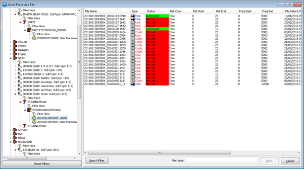
3. Once a manoeuvre is selected in the Database tree, all the processed files generated using the data from this manoeuvre are displayed in the list on the right hand side. Select the file then click 'Open' to display the default composite Zmod. (Below is a breakdown of the columns in this chart)
   1. Some files are available on disk and can be opened as soon as they are selected. Other files may need to be restored before they can be opened. When a restore request is made a confirmation is displayed and the user is notified once the data has been restored.
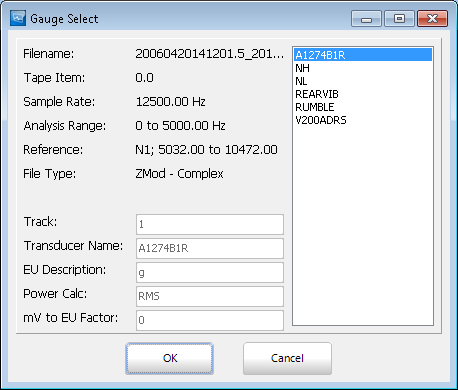
4. Once the file has been loaded, the 'Gauge Select' form is displayed, allowing selection from the channels found in the file.

Tabs in 'Open' Window

A number of fields of information are displayed for each processed data file in the open window.  These are:

1. File Name  –  this is the name of the file as it is stored in the HGL data analysis system.
2. Type – this will show the file type which can be Frequency, Complex Frequency or Time History
3. Status – this displays the Authorisation Status of the processed file.
4. Ref Chan – this is the reference data that has been used for the X-axis of the data in the file.  It is usually time or some form of test condition signal like a speed signal.
5. Reference Start – this is the start value of the reference channel.
6. Reference End – this is the end value of the reference channel.
7. Frequency Start – for frequency-domain processed files, this is the Y-axis start point, whereas for time-domain files, this value is always zero Hz.
8. Frequency End – for frequency-domain processed files, this is the Y-axis end point, whereas for time-domain files, this value is related to the sample rate of the processed file.
9. File Date & Time – this is the time and date when the file was created.
10. Group Map – this is the name of the Group Map used by the Aurora Tornado analysis module to generate the processed data file.
11. Proc Spec - this is the name of the Processing Specification used by the Aurora Tornado analysis module to generate the processed data file
12. User Name – this is the name of the user who requested the analysis reported in the processed data file.
13. Gap Type – this shows if the processed data file was analysed using a gapped or ungapped analysis method.

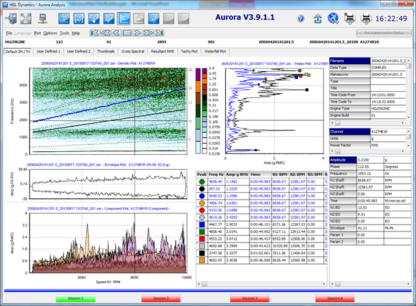
Data Viewer Overview

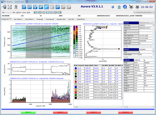
Once a file has been opened, Dataviewer will display the manoeuvres data on the screen. Below is an overview of the standard view in Dataviewer.

1. Engine Serial No
2. Test ID
3. Manoeuvre ID
4. Filename
5. Channel Name
6. Density Plot (Campbell)
7. Spectral Peak Plot
8. Channel Unit
9. Envelope Plot
10. Component Plot
11. Peak Table
12. First Channel
13. Previous Channel
14. Next Channel
15. Last Channel
16. Composite Plot Tab
17. User Defined Tabs
18. Cross Spectral Analysis Tab
19. Resultant RMS Tab
20. Tacho Plot Tab
21. Waterfall Plot Tab

Additional functions are accessed via right-hand (RH) mouse button menus

Displaying Different Channels of Data

There are 3 different methods for selecting which channel of data is displayed in Dataviewer. The channel can be picked from a channel list, picked from the Thumbnail display, and the channels can also be 'Played' through.

From the Channel List

1. To show the list of channels go to the top menu bar select 'Plot' > 'Select gauge. A new window will appear with the channel list. 
2. Select the channel you would like to view and click 'OK'

Thumbnail Display

1. From the composite display select the horizontal blue bar along the bottom of the screen. Use the scroll bar to view all the channels or resize the thumbnail pop up by dragging the border. 
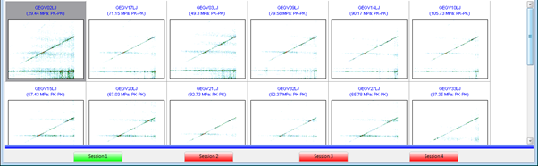
2. With the left mouse button, double click on the image of the channel to be viewed and the display will change to a composite plot of the selected channel.

'Playing' Channels

The play channels buttons are on the button bar at the top of the screen.

All the buttons have 'hints' attached to them, so if the cursor is held over the button for a short period of time a hint will appear to say what the specific function of the button is. 

1. The 'Play' button on the button tool bar, will cause the Dataviewer to play through the channels in turn at the current play rate The play rate may be adjusted by selecting the 'Options' > 'Select Scale...' menu option, and changing the 'Play Rate' setting.
2. The 'Stop' Button, will Stop the channels playing 
3. The 'First' Button, will display the first channel in the data file 
4. The 'Last' Button, will display the last channel in the data file 
5. The 'Previous' Button, will display the previous channel in the data file. 
6. The 'Next' Button, will display the next channel in the data file 

ZMod Plot Overview

1. ZMod/Density Plot 
2. Frequency Axis - Axis Start and End points can be changed via the right hand menu 
3. Time/Speed axis - Axis Start and End points can be changed via the right hand menu 
4. Amplitude - Colors represent amplitude using a log scale
5. Validation area - Area where data was marked invalid
6. Cursor - For more information on dataviewer cursors see the interrogation section below
7. Component Plot - more information on the component plot below
   1. Colored circles represent the highest peaks at the point of the cursor
   2. Colored squares represent the highest peaks of all the data
   3. By default this plot displays 10 peaks.

      ---

ZMod Plot Right Click Menu

1. Interrogate- is the default mode for Dataviewer, this mode allows you to click on any of the plots to display a cursor as well as zoom 
2. Edit Mode Lines- only available when reference channel is speed
3. Track Feature - Tracks a selected feature in the data
4. Simple Validation- uses a click and drag to select data for validation
5. Advanced Validation- gives options using engine order for the validation of data
6. Add User Defined Events- allows the user to highlight various types of events on a ZMod and attach a description. The user defined event is saved to a .xml file and is available upon reloading the processed file. 
7. Display Interrogate Cursor- turn off and on the cross hair cursors set in interrogation mode
8. Tacho Overlay- if a speed channel is in the data set you can overlay it onto the ZMod with this option
9. Overlay Tracks- turns on/off the track feature above
10. Reanalyse Using Zoom Window- allows the user to reprocess the data given the window they are currently zoomed in to
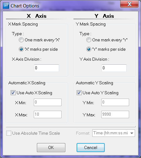
11. Chart Options- will display a pop up, in which the user can change the how the X and Y axis's are setup
12. Save to CSV- lets the user save the data to a CSV file either with the compact header or extended header.
13. Image Capture- gives the user the option to save images of the plot with 3 options
    1. print (default printer)
    2. export (saves to clipboard)
    3. save to file (.gif)

Interrogation Mode

The Interrogate mode is the default mode when Dataviewer is first started and can be selected from the Zmod plots right mouse button popup menu.

The cursor crosshairs are activated by selecting ‘display interrogate cursor’ from the ZMod right hand mouse menu. They are selected by default when in the interrogate mode. To place the crosshairs left click on the point of interest. 

A single shift-click action just outside the Z-mod plot area causes the cursors to jump to the maximum observed amplitude at a single frequency within a single spectrum.

ZMod Plot Cursors

1. Select 'Interrogate' from the density plot right hand side mouse pop up menu. Cursor cross hairs are displayed on screen. The interrogate table is updated showing cursor values at the center of the Z-mod. 
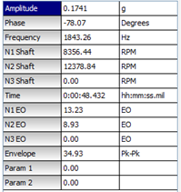
2. If a point is selected in the density plot with the Left Mouse Button for cursor interrogation the values at the cursor location are displayed in the interrogation table. The spectral peak plot display changes to display the single spectrum profile at the cursor location as well as the overview plot. and the peak table is updated. 
3. The cursor cross hairs can be moved using the arrow keys on the keyboard. The Interrogate box, the peak table and the single spectrum display will update.
4. Selecting a point for cursor interrogation with ‘Shift’ + Left Mouse Button in the density display will cause the cross hairs to move to the maximum value with in +/- 5 frequency bins and +/- 5 spectra of the cursor location.
   1. This allows the user to find the maximum peak value in a region of the plot without having to hunt manually for the maximum point in the data set.
5. The cursors can also be ‘Played’ by selecting the cursor play button on the tool bar and then the Play button.  This will move the cursor in the direction selected at the rate set in “ZMod Replay Rate” in the ‘Options > Set Scale’ window. 
   1. When the point was selected with the cursors in the density display the display in the peak plot changed to display a ‘single spectrum’ plot as well as an overview plot.  This is the output from the FFT analysis at a single value for the reference quantity, such as time or shaft speed. There are a number of options available to the user, which are accessed through a menu activated from the right hand mouse button when the cursor is in this window.

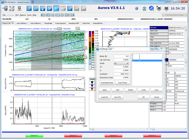
The ‘Edit mode line’ function allows the user to plot lines from quadratic equations of the engine speed onto the density plot.  The quadratic equations are then written out to a ‘Mode File’ where they may be used in other data processing utilities such as feature extraction.  The quadratic frequencies are based on frequency and speed values.

The ‘Edit Mode Lines’mode can be selected from the density plot Right Mouse Button pop up menu.

1. Once in the Edit Mode Lines mode, if the user double clicks in the density plot the mode properties box appears. 
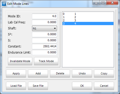
2. Selecting the 'Add' button will cause a mode line to appear on the density plot
3. The mode lines can be moved by selecting any of their three anchor points and dragging them
4. Details of the new mode can be entered into the mode window including mode label and endurance limits. 
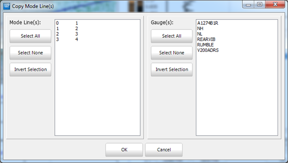
5. Mode information can be copied to other gauges by selecting the ‘Copy’ button in the mode box and specifying which modes you would like to copy across to different channels.  
6. The mode file must then be saved. This is done by selecting the 'save file' button on the edit mode lines form. A mode file will then be created containing the quadratic equation for the modes for each data channel.

Feature Tracking

Feature tracking is a tool in the HGL Aurora Dataviewer which allows the user to specify a feature within the data based on multiples of the reference channels and frequency and then to plot the values following that specific feature.  This option is available through the ‘Tools’ menu on the top menu bar.

1. If the 'Track Feature' option in the tools menu is selected the Track Options form is displayed 
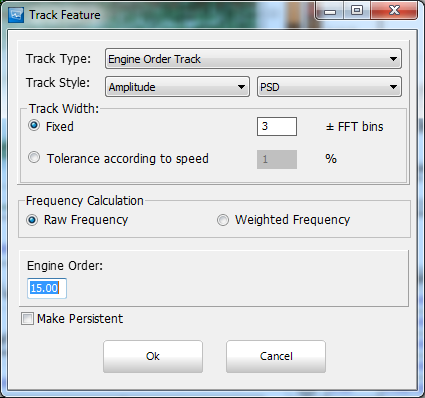
2. The detailed descriptions of all the available tracking options are located below
3. An engine order value can then be entered in the Track EO box and click the ‘Ok’ button. The tracked engine order will be plotted in the display area below the envelope display and the line of the track will be displayed over the top of the density display.
4. 'Track EO’ tracks a multiple of the reference channel. This option is only available when the reference channel is a shaft speed.
5. ‘Combined EO’ tracks the combined speed engine orders independently of the reference channel.  This is the option you would use to track a speed order if the analysis was against time.
6. ‘Track Mode’ tracks along a quadratic equation where Y is the frequency and X is the reference channel values of the analysis.
7. ‘Track Turning Point’ tracks a turning point defined by the user. It can be defined in terms of spectra and bin or freq and reference speed.
8. Multiple tracked responses can be displayed at any one time.

Tracking Style Options:

• Exact Style
  This plots the magnitudes exactly as requested by the user, along the exact tracking line defined by the user with no searching across neighbouring bins for higher values.
• Peak Style
  This looks for the largest peak by identifying clear turning points in the data and then finding the largest peak within the search range.  A peak value in this context is a value at a bin whose nearest neighbouring bins contain lower values. This is the most effective at finding clear resonance conditions with the lowest noise.
• Amplitude Style
  This looks for the largest amplitude in the data regardless of whether or not it is a clear peak within the defined search range.  This method is guaranteed to find the largest value but may be affected by any significant noise in the signal.  This option will be needed if a rising response occurs at the start or end of a manoeuvre.
• EO Style
  This ignores the search range defined by the user and tracks along the peak values closest to the Engine Order requested by the user.  This is a useful option when the bin width of the analysis is large.

Feature Tracking can be turned on and off in the right mouse button menu of the density plot by selecting 'Overlay Tracks'

Simple and Advanced Validation

The purpose of the data validation function is to tell Dataviewer if a specific spectrum of data is valid or invalid. The default setting for all data acquired through the HGL system is valid. When a range of spectra are set to be invalid, those spectra are ignored by all the plotting functions. Invalid spectra are not included within the peak-hold and average spectra plot options and are also not used when auto-scaling the amplitude axes of the plots.

Remark: This function is particularly useful for removing the effects of noise interference in the data as well as removing parts of the data that are of no interest.

The two validation modes ‘Simple validation’ and ‘Advanced Validation’ can be selected from the density plot Right Mouse Button popup menu.

Simple Validation

1. In the Simple Validation mode, if the Left Mouse Button is selected and the cursor is dragged over a range of spectra, when the user double clicks in the highlighted area, the Spectra Validation form appears containing a list of the identified spectra
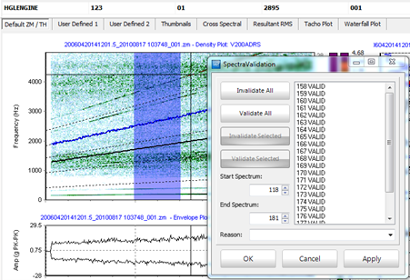
2. In the spectra validation window, if the ‘Invalidate All’ button is selected and then ‘OK’, all the listed spectra are marked as invalid. This is reflected in the density display by highlighting the invalid spectra in grey. The peak-hold plot is automatically recalculated and displayed using only the valid spectra. 

Once some spectra have been defined as invalid, it is possible to copy the invalid spectra flags across to other channels in the file.

Advanced Validation

Selecting 'Advanced Validation' from the density plot Right Mouse Button menu will cause the 'Advanced Validation' form to appear. 

This option enables the user to define a function along which data will be invalidated. It is possible to track an engine order, combined engine order or a mode and set a track width over which the invalidation will be applied. It is also possible to specify a range of spectra to further define the region to be invalidated.

Validation information is saved to an .xml file and is available upon reloading the processed file.

'Copy Validation Flags' can be selected from the 'Tools' option on the top menu bar. The Copy Validation Flags form then appears for selection of channels to which the validation flags should be copied. 

Dataviewer also includes an automatic validation function to detect noise and other poor quality indicators. This function will mark all spectra which are detected as being of poor signal quality as invalid. It is available in the 'Tools' menu.

User Defined Events

This option allows the user to highlight various types of events on a ZMod and attach a description. The user defined event is saved to an .xml file and is available upon reloading the processed file. 

When 'Add User Defined Events' is selected from the density plot Right Mouse Button menu the 'User Defined Events' form is displayed  

There are a number of User Defined Events or UDE types available;

Simple user defined event – the user defines a range of spectra to highlight.

Engine Order user defined event – the user specifies an EO to be highlighted, along with a range of spectra and width (in terms of +/- FFT bins).

Combined Engine Order user defined event – the user specifies a combined EO to be highlighted, along with a range of spectra and width (in terms of +/- FFT bins).

Mode user defined event – the user specifies a quadratic expression to define the mode to be highlighted, along with a range of spectra and width (in terms of +/- FFT bins).

When an engine order, combined engine order or mode has been specified a UDE style needs to be specified. The available options are exact engine order, peak, amplitude and engine order.

• Exact Style
  This plots the magnitudes exactly as requested by the user, along the exact tracking line defined by the user with no searching across neighbouring bins for higher values.
• Peak Style
  This looks for the largest peak by identifying clear turning points in the data and then finding the largest peak within the search range.  A peak value in this context is a value at a bin whose nearest neighbouring bins contain lower values. This is the most effective at finding clear resonance conditions with the lowest noise. 
• Amplitude Style
  This looks for the largest amplitude in the data regardless of whether or not it is a clear peak within the defined search range.  This method is guaranteed to find the largest value but may be affected by any significant noise in the signal.  This option will be needed if a rising response occurs at the start or end of a manoeuvre.
• EO Style
  This ignores the search range defined by the user and tracks along the peak values closest to the Engine Order requested by the user.  This is a useful option when the bin width of the analysis is large.

Once the UDE has been defined and added it is highlighted on the ZMod and if you hover the cursor over the event a pop up box appears displaying the name of the user who added the event and the description given.

Reanalyse with Zoom Window

Reanalyse with Zoom window allows the user to create another processing while zoomed in on a ZMOD/Density Plot.

1. In Dataviewer zoom in on the data of interest using the left click and drag 

   

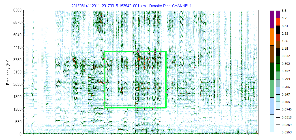
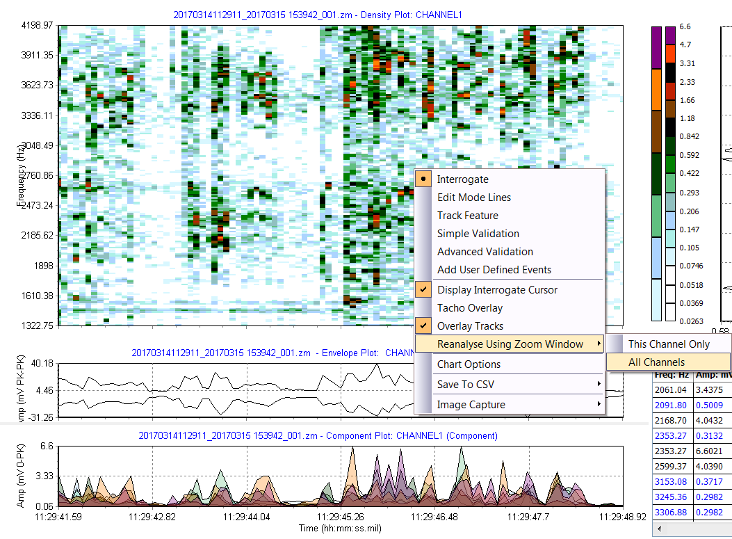
2. Once the desired window of data is achieved right click on the plot and under 'Reanalyse Using Zoom Window' the user has the option to either reanalyse the current channel or all of the channels in the processing.

   

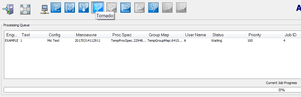
3. Once either of those options are selected, move over to the tornado, you can see the job has been created in the processing queue. 

   

4. When the job has finished processing it can be opened in Dataviewer, by navigating to the correct maneouvre in the open screen.

   ---

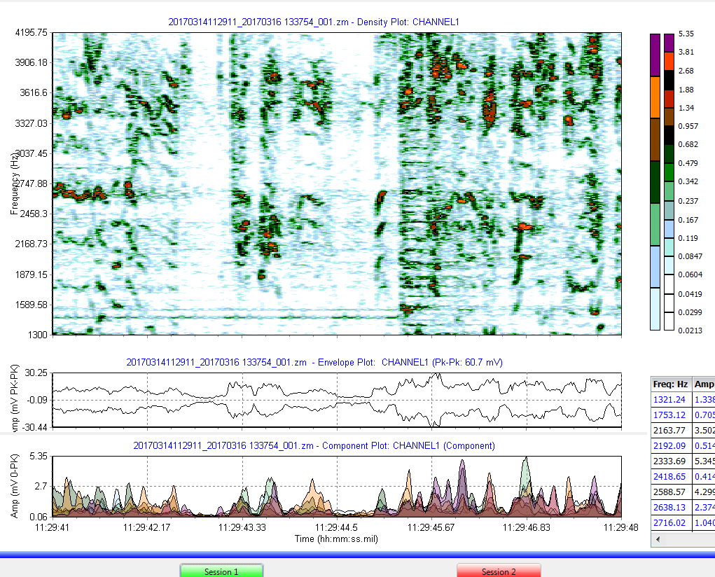
Chart Options

Chart options allows the user to adjust the X and Y axis spacing and scaling. Spacing gives the options of One mark per every X or Y or # of marks per side. Setting their numbers to 0 sets the spacing to their defaults.

X-axis and Y-axis Scaling - by default this is set to automatically scale but the user can turn off auto scaling and set the min and max of the axis to their desired values.

Lastly the time scale can be changed to use absolute time or relative time. Relative time is time from the beginning of the start of the processing or Absolute time being the exact time and date the data was recorded.

Save to CSV

Within the HGL Aurora Dataviewer, most of the plot types provide an option to write the plotted values to a file for later analysis and plotting in other programs. The output options are found on popup menus accessible via the right hand mouse button and allow the user to 'Save to csv'. The created files can be opened and viewed/edited in Excel.

Once 'Save to CSV' is selected the user will be able to save it where ever they would like.

ZMod Campbell Amplitude Scale

The main campbell plot (color density plot) on a ZMOD plot can become difficult to read if there is a single response that is significantly higher than all the other data points. When this happens, the plot will look washed out and faint.

This is fixed by changing the amplitude scale of the density plot, which can help to display a feature more clearly. 

Look at the menu bar at the top of Aurora, select "Options" >  "Scale Options". The following window will appear.

The top section sets the scale of the plot. The plot uses a color density system where a color is used to define an amplitude range, this is performed using a dB scale.

The "Scale Maximum" specifies when the last color range ends. If a plot needs to be darkened, choose a negative dB value (such as -10) as the "Scale Maximum". And, the reverse is true if the plot needs to be lighted; choose a positive dB value (such as 10). The default scale maximum is 0 dB.

The "Scale Range" specifies how much dynamic range there is for the color scale being used. A small dB value means there will not be a lot of colour variation in the plot because there isn't adequate separation. The default Scale Range is 48 dB.

"Num Levels" defines how many different colors are used for the amplitude scale. The defaults are either 8 or 16 and are typically defined by the selected colour map. Again, the more levels in the color map allows for greater dynamic range in the colour density plot.

It is also possible to modify the amplitude bands of the colour map via the component plot by dragging the edges of a segment, once moved with the mouse the numbers on the right will update to the new point that break point is at. Changing the colour of individuals segments is possible via a popup colour palette, that appears when a segment is clicked on.