
Dataviewer: Time History Overview
Time History Plot Overview
To view how to open a Time History processed file in Dataviewer perform the steps seen in ' Dataviewer - Overview'

- Envelope Zoom Plot
- Envelope Overview Plot
- Spectrum Plot
- Peak Tables
- Channel Navigation Buttons
Displaying Different Channels of Data
There are 3 different methods for selecting which channel of data is displayed in Dataviewer. The channel can be picked from a channel list, picked from the Thumbnail display, and the channels can also be 'Played' through.
From the Channel List
- To show the list of channels go to the top menu bar select 'Plot' > 'Select gauge. A new window will appear with the channel list.
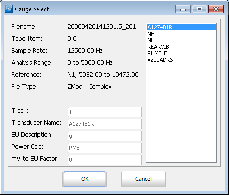
- Select the channel you would like to view and click 'OK'

Thumbnail Display
- From the composite display select the horizontal blue bar along the bottom of the screen. Use the scroll bar to view all the channels or resize the thumbnail pop up by dragging the border.
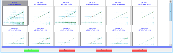
- With the left mouse button, double click on the image of the channel to be viewed and the display will change to a composite plot of the selected channel.

'Playing' Channels
The play channels buttons are on the button bar at the top of the screen.
All the buttons have 'hints' attached to them, so if the cursor is held over the button for a short period of time a hint will appear to say what the specific function of the button is. 
- The 'Play' button on the button tool bar, will cause the Dataviewer to play through the channels in turn at the current play rate
 The play rate may be adjusted by selecting the 'Options' > 'Select Scale...' menu option, and changing the 'Play Rate' setting.
 - The 'Stop' Button, will Stop the channels playing

- The 'First' Button, will display the first channel in the data file

- The 'Last' Button, will display the last channel in the data file

- The 'Previous' Button, will display the previous channel in the data file.

- The 'Next' Button, will display the next channel in the data file

 The play rate may be adjusted by selecting the 'Options' > 'Select Scale...' menu option, and changing the 'Play Rate' setting.


Octave Analysis
The Octave Analysis option is available when a time domain file is open. To open octave analysis select it from the top bar of Dataviewer.

Octave analysis enables the user to carry out a sound level measurement of a signal within the Time History module of Aurora Dataviewer. The frequency range is divided into a number of octaves: bands where the width of each band is twice that of the previous band. Calculation of the frequency bands is described in Appendix 1. For each octave, a specific filter is applied and the amplitude level is obtained by calculating the mean energy of the filtered data over a user specified length of time. 
On the octave analysis settings form the user can specify the order of the octave analysis, the minimum and maximum frequencies and the time range over which the analysis is to be carried out. 
The user selects part of the time history signal by swiping on the zoom plot. The amplitude level (linear or dB) is then displayed on a histogram for all octaves, with frequency values displayed on a logarithmic scale. The octave frequencies are determined from a reference centre frequency of 1000 Hz and the user can choose the number of octaves to be included in the analysis by selecting the desired lower and upper bounds from a drop-down box. X-axis labels can be also toggled between frequency values and frequency band indexes.
It is possible to zoom in on the octave plot by holding down the left mouse button and dragging down to the right.
Right Hand Mouse Menu

- Select Channel - Brings up channel selection page
- Octave Analysis Settings - Brings back up Octave analysis settings
- Chart Options - Brings up options to adjust axes
- Show Frequency Band Indexes - switches between showing frequency band indexes and frequency values
- Display Bars on Log Scale
- Save to CSV
- Image Capture
- Print (default printer)
- Export (Clipboard)
- Save to File (.Gif)
Averaged FFT
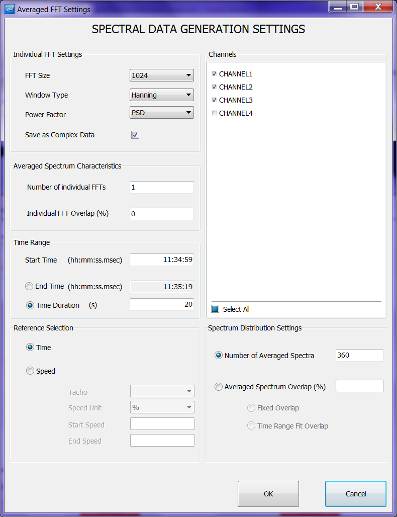
This feature is for performing an averaged spectrum with various calculation options, for a set of user-selected channels, and over a user-defined time range.
The Averaged FFT Settings dialogue appears the first time when clicking on the Averaged FFT tab, or through the main menu (Tools -> Averaged FFT)

- FFT Settings
- FFT Size - changes the size of the FFT
- Window Type - Options are Hanning, Hamming, Blackman
- Power Factor - Options are 0-pk, pk-pk,RMS, and PSD
- Average Control Mode
- Number of FFTs - you can specify the number of FFT's the average will be performed on
- FFT Overlap
- Fixed Overlap - percent overlap
- Time Range Fit Overlap - the overall overlap will be adjusted in order to cover the last samples in the time range for the calculation
- Time Range
- Start Time defaults to start time of manoeuvre but can be adjusted
- End Time defaults to end time of manoeuvre but can be adjusted
- Time Duration - length of averaged FFT
Display

The spectra appear on the Averaged FFT Plot. In the legend, click on the channel name of interest in order to lock the cursor to that channel.
Right-click Menu

- Averaged FFT Settings - Brings back up the averaged FFT settings
- Switch to Transmissibility Plot - Switches to the Transmissibility Plot, covered in next section
- Generate Wavelet File - Brings up Wavelet File Generation menu

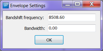
- Envelope Spectrum - Brings up Envelope Settings
- Chart Options
- Generate Spectral File
- Save to CSV
- Image Capture
- Print (default printer)
- Export (Clipboard)
- Save to File (.Gif)


Transmissibility Plot
The transmissibility plot is accessible from the right-click menu of the Averaged FFT plot, on the Averaged FFT tab for Time History files. When selecting that option, the Averaged FFT page switches to show the Transmissibility plot. This plot display the transmissibility spectra averaged over multiple FFT's, like the Averaged FFT.
Display

Right-click Menu

- Transmissibility Settings - Settings are shown in the next section
- Switch to Averaged FFT Plot - Switches back to the Averaged FFT page
- Chart Options - Brings up options to change scaling of axes
- Save to CSV - outputs data to .csv file
- Image Capture
- Print (default printer)
- Export (clip board)
- Save to file (.GIF)
Settings

The settings are accessible via the right-click menu from the Transmissibility plot. They are similar to the Averaged FFT Settings
Wavelet Analysis
Wavelet Analysis files are frequency/time domain data files where data are stored in a format that complies with the New HGL File Format Schema. They provide the ability to analyse a TH file against a decomposition function called wavelet, that are defined functions the user will choose prior to performing the analysis.
Generating Wavelet Files
Wavelet files are generated from the right-click menu of the Averaged FFT tab that you can access when you opened a Time History file.
Settings
The setting dialogue form appears when selecting option Generate Wavelet File. 
Section: Wavelet Analysis Settings
This allows the user to choose the wavelet to use for the wavelet analysis and the size of the block the analysis will be done.
Section: Time Range
Define the time region over which the wavelet data must be generated. The time region can be defined graphically from the Envelope plot on the Averaged FFT page.
Section: Reference Selection
For the moment, wavelet analysis file can only be generated using time as reference.
Section: Channels
Allow the user to select the channels on which the analysis will be done.
Viewing Wavelet Files
From the main menu click on File → Open HGL Files (Spectral, Wavelet…). Browse the tree view to the desired location and select your file. The name of the file will be slightly different, as a timestamp has been added as a suffix when it was created. 
Your wavelet file data will be display as a simplified ZMod data file on the Default ZM page. 
Strain Rosette Analysis
If you opened a time history file, you have access to a strain rosette tab. This tab provides a strain rosette analysis method.
The first time you click on the strain rosette tab a settings pop up window will appear, to bring up the strain rosette settings after the first time can be done in the 'Tools' menu and selecting Strain Rosette. 
In the upper section of the pop up select the geometry of the strain rosette used during the test:
- Rectangular (i.e. with 45 degrees between the gauges)
- Delta (i.e. with 120 degrees between the gauges)
The lower section defines which gauge corresponds to which value according to the geometry schemes. Once the 3 gauges defined, click 'OK' to display the values.
Strain Rosette Values

The 3 plots displayed are:
- The principal strains against X and Y on the top plot
- The angle against the rosette axis on the middle plot
- The shear strain on the bottom plot
The operations of zoom-in and zoom-out are available and the 3 plots are linked so a zoom operation on one plot will be applied on the others.
Remark: Zooming operation will provide either a one point-per-pixel resolution or provide envelope values for a slice of data per pixel if the amount of data is too big.
Rainflow Analysis
This menu option is active when time history data is displayed and provides the facility to cycle count a section of data for further fatigue analysis. The cycle counting method used is the ‘range-pair’ method as defined in ASTM E 1049 –85, ‘Standard Practices for Cycle Counting in Fatigue Analysis’.
- Select the ‘Rainflow’ option from the Tools menu, this produces the user input screen for the rainflow analysis.
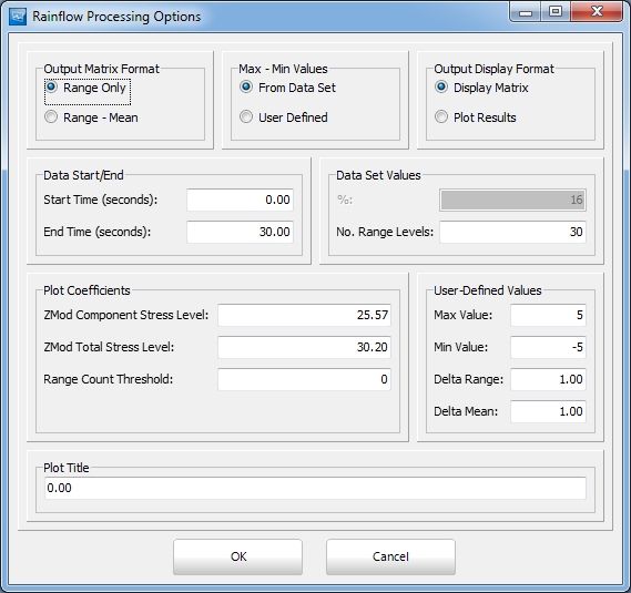
- Select a Range-Mean count, use max-min values from the data set and select to display a matrix.
- Enter appropriate start and end times and select OK.
- The Rainflow Matrix is displayed
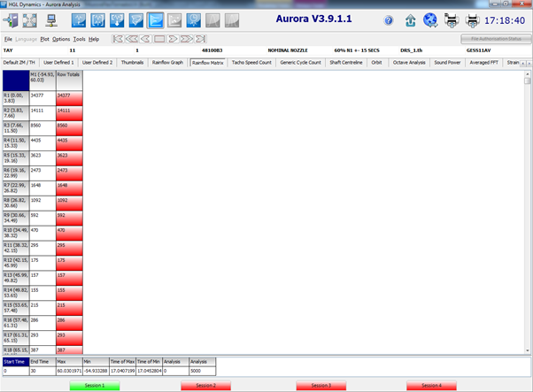


It is also possible to plot rainflow results or carry out a range only analysis.