
Dataviewer: Other Plot Types
Peak Plot

- 'Overview’ will display the peak hold plot. This displays the maximum value detected for each frequency bin across all the spectra, any spectra marked as invalid will not be included in the peak hold calculations.
- 'Single Spectrum’ will display the peak hold plot. This displays the spectrum value along the vertical axis of the cursor on the density plot.
- ‘Average spectra’ will display the average response along each frequency bin. This gives the average frequency content over a period of time and should only be used when the vehicle from which the data set was acquired was at a steady state condition. Any spectra which have been marked as invalid will not be included in the average calculations.
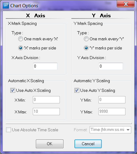
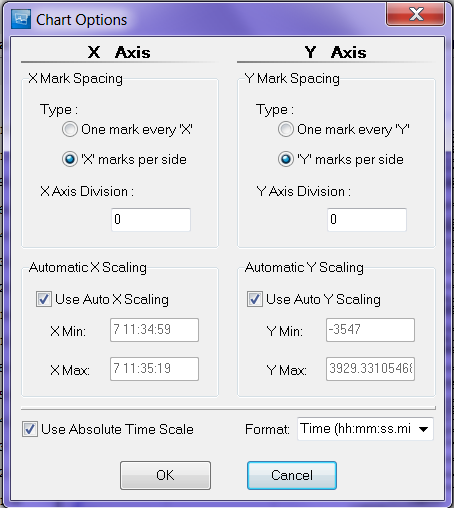
- 'Chart Options' will display a pop up, in which the user can change the how the X and Y axis's are setup
- 'Save to CSV' lets the user Save the data to a CSV file either with the compact header or extended header.
- 'Image Capture' gives the user the option to save images of the plot with 3 options
- print (default printer)
- export (saves to clipboard)save to file (.gif)

Peaks Table

The peak table is the bottom right plot in Aurora's Dataviewer The chart displays the max peaks from the zoom window displayed as squares as well as circles representing the peaks from the cursor on the ZMOD plot. By default 10 peaks are displayed, each peak shows its amplitude, time, tacho, and engine order information.
Right clicking on the peak plot brings up the following options.
- Mode
- Peak Table
- Tracks
- Save to CSV
- Image Capture
- Printer (default printer)
- Export (clipboard)
- Save to file (.gif)
- Time Format
- (hh:mm:ss.mil)
- Seconds
- View Row/Column
- disable unused columns or add in columns
- Sort by
- Select Ascending/descending and select column

Envelope Plot

- Standard Envelope - shows the positive and negative
- Total Vibration (pk-pk)
- Chart Options - Allows user to adjust scaling of X and Y axis as well as the spacing of the tick marks for the scale
- Save to CSV - Saves plot data to a .csv file
- Image Capture
- Print (Default Printer)
- Export (Clip Board)
- Save to file (.GIF)

Component Plot

- Component - displays multiple bins of data over top each other
- Single Bin - displays a single bin of data
- Tacho - displays the tacho
- Broadband
- Full Bandwidth
- User Selectable Bandwidth
- Param
- Track - Displays tracked order
- Performance
- Chart Options
- Performance Settings
- Save to CSV - saves plot to the .csv file
- Image Capture
- Print (Default Printer)
- Export (Clip Board)
- Save to file (.GIF)
User Defined Displays
On the 'User defined' screens it is possible to create a display configuration using the available components. When first selected a blank screen is displayed with various options down the right hand side.
 If the user selects one of the components from the 'Create Components' list, with a left mouse click the selected blank component appears on the screen. It is possible to resize the component by dragging its corners or edges and it can be moved and re-positioned on the screen by dragging it to the desired location, holding down the left mouse button.
 Once all the desired components have been selected, resized and positioned on the screen select the blue horizontal bar along the bottom of the page to populate the plots with data from the processed file currently open, and the various selection tools down the right hand side of the screen disappear.
 The various components can be linked in a number of ways, using the component management option. Selecting the 'component groups' button causes the 'Component Group Management' form to appear.
Component Group Management
Various components can be linked in a number of ways, using the component management option. Selecting the 'component groups' button causes the 'Component Group Management' form to appear.

If the user selects ‘new component group’, 'Component Group 1' appears in the window on the left hand side of the form. The user then needs to select components to make up this group. This is done by selecting components on the screen with the left mouse button, whilst holding down the ‘ctrl’ key. The user then selects how the selected components within the component group are linked. The available options are channel, cursor, zoom area or data mode display.
It is possible to save user defined configurations and reload them at a later date and with other compatible files. Load, save and save as options are available under the ‘standard’ menu down the right hand side of the screen.
Following is an example of how component group management could be used for a time domain file.
Open a time history file and select one of the user defined tabs. Using the ‘create components’ options create a new layout which has a time history envelope plot across the top of the screen and two smaller envelope zoom plots adjacent to each other directly underneath. Underneath each zoom plot create an fft plot.

Using the ‘component management’ options create a component group which includes the envelope overview plot and the two envelope zoom plots, linked by zoom area. Another component group including one zoom plot and the fft plot directly under it, linked by channel and cursor. The final component group should include the other zoom plot and the fft plot directly under it, again linked by channel and cursor.
Click on the blue horizontal bar along the bottom of the screen to populate the plots. Selecting a zoom area in the overview plot will update the zoom plots and fft plots. From the right mouse menu on one of the zoom plots select a different channel. The zoom plot and linked fft plot will update to display data for the selected channel over the zoom area selected in the overview plot. i.e. this plot layout can be used to select the zoom area on data for one particular channel and simultaneously view data for two different channels over the same zoom area.
 The user defined layout is saved to xml file and is available upon reloading the processed file. Persistent workflow xml files are created during the analysis process when major operations are carried out;
- tracking is carried out
- validations are performed
- user defined events are created
- unit or power factor conversions are performed
- colour map and scale options are selected
- data manipulations carried out
- parameters derived
The data created during each of these operations is then available when the processed file is reloaded.
The xml files are stored next to the appropriate processed file and can be copied or deleted as required. The processed file name is used in the xml file naming convention so the appropriate xml file can be easily identified.