Rawviewer: Overview

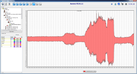
To view data in Rawviewer first launch Aurora Client. Rawviewer editor is the eighth blue square icon in Aurora Client, and is used to look at the raw data without any processing. This allows the user to quickly look at the data from a manoeuvre to see trends or spikes in the data where a potential problem occurred.

Plotting Data

1. The user must first select the data to display by the selecting the Manoeuvre of interest from the HGL database tree view in the top left hand corner of this display.  
2. Once a manoeuvre is selected the channel grid, below the database tree will be populated with all the channels available for the selected manoeuvre. 
3. Check the channels of interest, their data will appear on the plot to the right. 

Adjusting Zoom and Panning

It is possible to zoom in and out of the displayed timeline as well as being able to pan (move forwards and backwards through the time line).

Zooming In - To zoom in drag the left mouse button from the top left to bottom right, creating a zoom box around the region of interest. The zoom box will zoom both amplitude and time line.

Zooming Out - Zooming out is performed in the opposite fashion as zooming in. Drag the left mouse from bottom right to the top left, the amplitude will automatically scale so that the highest peak is the full scale point.

Panning - To pan the current viewing window of data hold the right mouse button drag left or right to pan the time line or drag up and down to pan the amplitude.

Remark: Zooming operation will provide either a one point-per-pixel resolution or provide envelope values for a slice of data per pixel if the amount of data is too big. 

Changing Time Axis

Real time, Pseudo time, Speed

There are three option to display your raw plot, Real time, pseudo time and speed. This options modifies the plot to show you the data against the real time, pseudo time or speed. Data can only be displayed against speed when there is a presence of a tacho.

Create manoeuvre mode

Create manoeuvre mode allows the user to create a manoeuvre directly from rawviewer. To access Create manoeuvre mode right click in the plot area and select it. Now highlight the data of interest on the plot by using the left mouse button. Once the mouse button is released a box will appear where you can adjust the start and end times, give a description, type, and tape item. When all the details are set click create and the manoeuvre will be created. 

Note: The start and end time will snap to the nearest whole second.  

Interrogation

Choosing Interrogation from the right click menu will bring up the box shown below. The interrogate box will allow the user to select whether they wish to interrogate Raw data or processed data. Once the mode of the interrogate box has been selected it will then display the amplitude information from the selected data type for all parameters that are being displayed and that have coincidental points. The cursor itself is represented by a Lime Green vertical line. 

Chart Options

To adjust the chart options right click on the plot in Rawviewer and select chart options. The chart options dialog allows configuration of chart axes, margins, legend and title.  

Under the chart tab the user has the option to give the plot a title, legend, and adjust the margins. The box to edit the title become editable when the visible box is checked. The title does not have length restrictions.

Margins can be adjust for the plot by either pixels or by percent. 

  In order to display many parameters on the screen simultaneously it can be useful to use multiple axes so that parameters with similar amplitude ranges are grouped together. Creating new axes is achieved by creating parameter groups and associating each parameter group with a particular axis. For example, all temperature parameters could be designated as belonging to parameter group “Temperatures” and all speed parameters could be designated as belonging to parameter group “Speeds”. The “Temperatures” group could then be linked with the LH axis and the “Speeds” group could be linked with the RH axis, maximizing screen usage. Parameter linking is shown here: 

1. Add a New Parameter Group by clicking on the ‘Add Parameter Group’ button, a new dialog box is displayed in which the user types the name of the parameter group
2. Select the Engine whose channels are to be configured from the drop down to populate the Parameter grid (the parameters that are then displayed are those channels that are currently being displayed for that Engine in the main Analysis window).
3. The parameter group for a listed parameter can be modified by double clicking on the listed parameter group and selecting a different one from the drop down list which appears. 

Once the parameter groups have been defined, the axes linking is done on the axes tab as shown to the right. From here properties of each axis can be configured as the user desires.

1. New axes are created and parameters linked from the ‘Axis Linking’ section. Select the Parameter Group to configure from the left hand drop down menu and select the location for the new axes, performing the selection instantly creates the new axes and relocates the parameters to it based on the parameter grouping.                                                                                                                                                                                                                 NOTE: the graph can have up to 12 separate axes, 2 axes wide, 3 axes high and on both the left and right hand side of the plot
2. Specific axis options are configured from the ‘Axis Configuration’ section. Select the axis to configure from the drop down menu and then make the changes to the axis properties from the ‘General’ and ‘Scales’ tabs. The General tab allows the user to set a label for the axis, turn the grid on and off, and to change the axis offset (i.e. its distance from the plot). The Scales tab allows the user to configure the scale and range of the axes. 

Once the user has configured the parameter grouping and axis linking, the configuration can be saved via the ‘display Configuration tab’. Note the saved information includes the data set and time segment that is currently displayed so that loading a configuration returns the program to the exact same state as it was in at the time of the save. 

Export to Matlab

You can export the data to matlab by right clicking on the plot and selecting 'Export to matlab'. This brings a side pull out menu that gives 2 options. 

All Channels - exports all channels from the maneouvre into matlab

Selected Channels - exports all channels being displayed from the maneouvre into matlab

Save to CSV

The Save to CSV option will create a CSV file containing data for either 'All channels' or the currently 'Selected channels only' for the time frame of the current view of plot. If the plot is zoomed only that time frame will be included. 

Export to DATX

You can export the data to DATX making right click on the manoeuvre and selecting Export to DATX, then you can choose the channels that you want to export to DATX. 

Once you decided which channels you want to select ( All channels…, Selected channels only… or Multiplex), a popup window will appear to choose the folder where you will keep your DATX index file and DATX file. Select 'OK' once the folder is selected.